Polyphonic pickup, measurements
repository: polypu
With coils in hand, and lofty ambitions about system performance in mind, we can now orient ourselves towards building and optimizing circuitry to reify some of our imaginings. However, keeping the old principle in mind that we cannot improve what we cannot measure, we would do well to pour some time into establishing and refining our own methods of measurement first.
To define where we are headed, let’s take the simplest requirements that our circuit will ultimately have to satisfy: the differential amplification and digital acquisition of six input channels. There are many metrics we could judge the circuit by, but the most important are probably the per-channel and total signal-to-noise ratios, the levels of crosstalk between channels, and the frequency response within the audible range. There are also requirements towards external connections, power draw, manufacturability, expectations towards component ICs, as well as total cost, but those will be secondary until some evidence of feasibility is found.
I’ll try to avoid mixing the software-wise implementation in here as much as possible, unless it is important, interesting, or hardware-specific. For the time being, I’ll grab an ESP32-S3 MCU and an MCP3008 ADC to start with, and we’ll see how far they can take us in these experiments.
Analog-to-digital converter specifications
The datasheet for the MCP3004/3008 chips specifies a resolution of 10 bits, and a sample rate of 200kHz. The latter is only guaranteed with a supply voltage of 5V, and it falls to 75kHz with a 2.7V supply. If we consider each bit to expand our dynamic range by roughly 6dB, the bit depth gives us a dynamic range of roughly 60dB, which may not be enough for usual audio purposes - and even less so for precision measurements - but let’s try to make that useful for as long as possible. For the sake of accuracy, computing the SQNR (signal-to-quantization-noise ratio) for 10 bits comes out to be 61.96dB, according to the following formula.
20 * log_{10}(\sqrt{1.5} * 2^{bits})As for the sampling rate, we’ll have to rig up a demo to find out the actual maximum rate that the hardware and software of our microcontroller will let us make use of, as there can be multiple bottlenecks keeping us from reaching the maximum sampling rate of the ADC.
After studying the serial interface timing for the communication that will happen on this SPI bus, initializing the bus for usage, and verifying that we can send and receive data as part of a transaction, let’s find out the repetition rate of this transaction by sending one right after another, and measuring the time between their starting points. The transaction length here was configured to be 18 bits, matching the length of the actual communication, rather than padding it to 24 bits / 3 bytes as the firmwares of some microcontrollers do.
esp_cpu_cycle_count_t start = esp_cpu_get_cycle_count();
spi_device_polling_transmit(SPI_DEV, &SPI_TRA);

ELAPSED = esp_cpu_get_cycle_count() - start;
spi_device_polling_transmit(SPI_DEV, &SPI_TRA);
The only quirk here is that if we use a simple printf(),
printing has to happen outside of an ISR context, as, for instance, my
code happened to issue and measure these transactions from the callback
of a timer. As for the elapsed time, we get a stable 2876 cycles, and
dividing by the 160MHz the processor was running at, we get 17.965us for
the repetition delay, which amounts to a maximum repetition rate of
55.632kHz.
To verify the accuracy of this measurement with a scope, I placed two cursors on the falling edges of these two transactions on the chip select pin, and the time between them was 17.68us, which amounts to a repetition rate of 56.561kHz. While the overhead of roughly 45 cycles is noticeable, it is also possible to counter by measuring and subtracting it from the results, and it also diminishes considerably with optimizations enabled. The point is that while it’s nice to have a scope for these things, measuring this delay is definitely possible with just cycle counts.
To be fair to the stock drivers, I also made these measurements again
after compiling with -O2. Note the decreased overhead of
getting the cycle count.
| method | clock cycles | microseconds | kHz |
|---|---|---|---|
| cycle timing, -O0 | 2876 | 17.96 | 55.632 |
| oscilloscope, -O0 | 2831 | 17.68 | 56.561 |
| cycle timing, -O2 | 2633 | 16.46 | 60.767 |
| oscilloscope, -O2 | 2630 | 16.44 | 60.827 |
Either way, once we start contemplating 60kHz as the maximum frequency, we could be forgiven for shaking our fists at the firmament and cursing the stock SPI drivers. Even when clocking the bus at the recommended 3.6MHz - making transactions shorter relative to the delay between them - this is nowhere near the 200kHz that our ADC could theoretically provide!
The reasons for this limitation seem to be twofold: as far as I could tell, the concept of a transaction in the high-level SPI driver interface provided by esp-idf implicitly includes a single pair of edge transitions on the chip select pin, which collides with the protocol defined by the MCP3008, wherein the chip select line must return to a high state between transactions. This means suffering the processing delay of the stock interface upon every transaction.
Looking at the implementations of
spi_device_polling_transmit() and the functions it calls,
it might start to become apparent why they take so long to repeat
identical transactions. They were built for a lower common denominator
of assumptions, wherein they put fewer constraints on the types of
transactions and on the code that may run between and outside of those
transactions in exchange for having to repeat more setup code each time.
In contrast, the transactions in our situation are not only nearly
identical and repetitive, they also complete in a time that is a good
bit shorter than the overhead of sending them, which more than halves
their effective data rate.
While this frequency may be fine for something like sampling a single audio channel at 48kHz, there are motivating reasons to target a higher frequency in these experiments: we could either increase our bandwidth (and get a better idea about the high-frequency content of the signal), or we could oversample (to improve resolution and to reduce noise).
Refactoring the high-level SPI drivers
Towards the end of the previous section, the conclusion was that the crux of the problem is how the stock drivers set up every aspect of the transaction each time, even if only the transmitted and received bytes vary between them. At least, that seems to be the case for the polling interface. I haven’t tested the interrupt/queued interface, as it seems less relevant for sampling an audio channel at an exact frequency, and it doesn’t seem like it would be much different in this regard either.
Knowing this, why don’t we try changing the drivers? After all, we have full access to a local copy of esp-idf, and we only have our time and sanity to lose. The code may be labyrinthine and haunted by a proportionate madness, but here’s the thing: we don’t need a full understanding of what it does to trim away the portions that are unnecessary to repeat between (nearly) identical transactions.
If we have a way of verifying that the correct communication takes place while using our replacement interface that omits unnecessary portions (and hopefully only those), we can keep bouncing back and forth between breaking/retaining functionality until we end up with a slimmer interface suitable for repeating transactions. While this isn’t an easily portable solution, it can work in this situation, where only a single SPI driver is used for this singular purpose.
The interface I ended up implementing has three functions. Two of
them are minimal versions of the two functions that start and end a
polling transaction, and a third one tries to repeat-start a transaction
that was configured earlier, assuming that nothing significant has
changed in the meantime. These functions are implemented in
esp32s3/main/spi-custom.c.
esp_err_t IRAM_ATTR spi_custom_polling_repeat(
    spi_device_handle_t handle,
    spi_transaction_t* trans_desc,
    spi_hal_trans_config_t* hal_trans
){
    spi_device_t* dev = handle;
    spi_host_t* host = handle->host;
    spi_hal_context_t* hal = &(host->hal);
    spi_dev_t* hw = hal->hw;
    spi_hal_trans_config_t* trans = hal_trans;

    //Set polling, no interrupt used
    host->polling = true;

    //Set current device doing the transaction
    host->cur_cs = dev->id;

    //Clear int bit
    spi_ll_clear_int_stat(hal->hw);

    //Need to copy data to registers manually
    spi_ll_write_buffer(hw, trans->send_buffer, trans->tx_bitlen);

    //Start user-defined transaction
    spi_ll_user_start(hal->hw);

    return ESP_OK;
}
I’ve included the above code only to show how little the repeater function has to do to send off another transaction, at least in this specific constellation of hardware and software. All that remains is to set up the interface by issuing our versions of the starting and ending functions once, on initialization. Measuring the transaction delay again shows a considerable improvement in the repetition rate of the interface.
| method | clock cycles | microseconds | kHz |
|---|---|---|---|
| cycle timing, -O2 | 1167 | 7.29 | 137.174 |
| oscilloscope, -O2 | 1164 | 7.28 | 137.362 |
Implementing measurements
After the above demonstration, it was time to start resuscitating the software by laying the necessary pipework for the next function, and measurements seemed like a decent piece to add back into the picture. Here, I would like to go over the approach briefly, and to sprinkle in a few technical details.
Since I wanted to make measurements while the device is running in a steady state - to avoid any concerns about delaying and disrupting execution while allocating and initializing any particular measurement - I have made the allocation and freeing of resources separate from the actual measurement in the command interface. This time around, I also put the measurement functions behind common function typedefs, which helped remove a lot of boilerplate that grew with every newly added measurement type in the past.
The results of a measurement were sent out over the USB-OTG
peripheral of an ESP32-S3, configured to act as a USB CDC-ACM device
(communication device class, abstract control model). The data itself
was in the printable ASCII range, and two extra characters called DC1
(0x11) and DC2 (0x12) were used to mark the
beginning and end of a transmission. These characters were caught by a
short program in C that was responsible for setting up the communication
port and extracting the data to be received. Finally, a short shell
script automated this flow of actions, and invoked gnuplot to graph the
results.
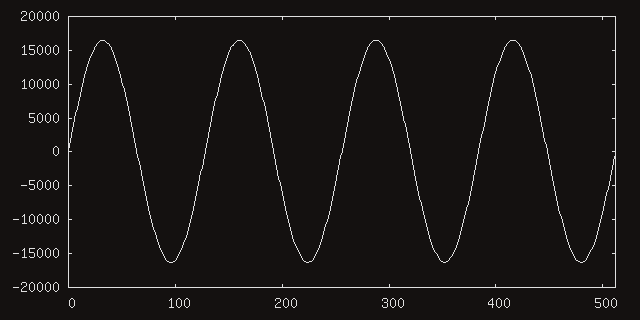
The above measurement is the first and possibly the least complicated, as it just outputs a series of samples from a single channel. Although more complex measurements will become necessary later on, this can already be useful for sanity checks.
A technical tidbit that may be worth mentioning has to do with
writing to a CDC device with tinyusb. When shoveling data to be written
by the metric ton, interspersing write calls with flushes and making
sure that the tinyusb task executed regularly was somehow never enough
in my setups to get all data to be sent, in the correct order, with no
skips in between. When we approach the maximum buffer capacity or
bandwidth of the underlying channel, there has to be some sort of flow
control if we want to avoid losing data. Thankfully, tinyusb provides
the tud_cdc_n_write_available function, which lets us check
how many bytes the output fifo could still receive.
Frequency spectrum measurement
The next measurement will be one of the most useful for evaluating
noise performance: a frequency spectrum, obtained by taking a sequence
of samples and applying a fast Fourier transform (FFT) on them. Here,
I’m using the kissfft library with complex input and output
signals, and with a uniform window. In the following, I’ll be working
with a complex signal, even though the library provides an interface for
real signals as well, which should run faster and with less memory. I
still have to figure out how to normalize the results of that interface
correctly, as they seemed to be -3dB lower for some reason.
First, the input signal should be converted to a complex signal by
assigning the sample value to both the real and imaginary components at
each point. After applying the transformation, the first half of the
complex output signal will contain values that can be interpreted to be
representing the frequency components of the signal from DC to half the
sampling rate (called the Nyquist frequency). To convert a single point
x of the result to a level in dBov (decibels overload), we
first compute its euclidean norm.
float norm = sqrt(x.r * x.r + x.i * x.i);Then, we normalize the result through dividing it by the signal length. This is a part which seems to be correct, but since I don’t yet understand how it relates to power spectrum and power spectral density, I couldn’t tell you why.
float normalized = norm / length;Finally, we express the ratio as an amplitude ratio, or root-power quantity.
return 20. * log(normalized) / log(10.);To verify the correctness of the measurement, let’s generate a test signal by combining a half-amplitude sine wave (generated in software) with the slight noise of a voltage buffer (measured by hardware).
The frequency of the sine wave is 375Hz, to center it on a result bin that has exactly that frequency (to avoid any scalloping loss, which could be as high as -3.92dB with a uniform window). That frequency was chosen based on the sampling rate of 48000 and the 65536 value range of a 16 bit integer. Their greatest common divisor is 128, and if we take this to be the sample interval of one cycle, we get 375Hz. The voltage buffer is just buffering a half-voltage, and it produces a hundred or two values of noise fairly close to zero. The window length is 8192 samples.
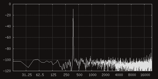
After measuring the spectrum, we get a peak of -9.03dBov at 375Hz, and low-amplitude noise everywhere else. This seems correct, if we remember that a full-scale sine wave should be -3.01dBov, and that halving the amplitude is equivalent to a -6.02dB reduction.
Ghosts in between the machines
Lastly, I want to mention some bizarre behavior I’ve found around communications over USB, an issue that almost drove me insane some months ago, and which took two hours from my life again just recently. While trying to receive data from longer measurements over CDC, I noticed that some portions of the transmission were dropped at random. The code itself hardly could have changed, as I was just getting ready to get something done on the project that day, and everything was working just fine the previous day. I spent ours trying to figure out if I was misusing the CDC interface somehow, but to no avail.
Then, as I stared at the cables coming off of my breadboard, I noticed it: my phone was also plugged into the front panel of my desktop, to charge. Even without interaction, it was evidently communicating something with the host, or at least it was trying to, and that interfered with the exchange happening on the cable going into the USB-OTG peripheral on the devboard. Both were USB 2.0 ports, by the way, and the problem seemed to disappear after plugging the latter cable into a USB 3.0 port on the same front panel. Really makes me wonder just how much hardware is shared between those two USB 2.0 ports. I’ll leave taking apart my machine far enough to find out for another day, though.
created
modified